Analyzing the Hyperplonk Proof System, a Hardware Perspective

The Cysic team would like to thank Luke Pearson and Binyi Chen for valuable feedbacks on this post.

Hyperplonk is an adaptation of the Plonk proof system to the Boolean hypercube that aims to eliminate the need for computing fast Fourier transforms (FFT) during proof generation. It also supports custom gates of higher degree without increasing the proof generation time.

In this article, we will analyze the performance of Hyperplonk from a hardware perspective, focusing on the pros and cons of its three computing components: multi-scalar multiplication (MSM), multi-linear extension (MLE), and sumcheck. We will also propose our design for these components and potential improvements to Hyperplonk for better performance on customized hardware.

Overview of the Hyperplonk Proof System

Hyperplonk is a type of succinct non-interactive argument of knowledge (SNARK). One of the most important features for SNARKs is succinctness, which means that the size of the proof depends logarithmically on the size of the circuit being proved and the verification time is proportional to the length of the statement plus the logarithmic size of the circuit. There are two primary components in constructing SNARKs: an interactive oracle proof (IOP) and a cryptographic commitment scheme:

• An IOP is an interactive proof in which the verifier does not need to read the entire proof, but has oracle access to the proof script and can probabilistically query it.
• A commitment scheme functions similarly to a sealed envelope, hiding and bounding the message inside it at the same time. Commitment schemes, such as KZG, FRI or Merkle tree, are widely used.

The common paradigm for obtaining a SNARK from an IOP and commitment scheme is to compile the proof in the IOP using a commitment scheme.

There are three categories of SNARKs based on different flavors of the IOP and commitment scheme:

• Polynomial-IOP + univariate polynomial commitment scheme
• Multivariate-PolyIOP + multilinear polynomial commitment scheme
• Vector-IOP + vector commitment scheme

Hyperplonk belongs to the second category, while Plonk belongs to the first one. It is also possible to add zero-knowledgeness to SNARKs to obtain zkSNARKs, but for simplicity, we will not analyze the zk-Hyperplonk scheme in this article.

The key difference between Hyperplonk and Plonk is that Hyperplonk works on the Boolean hypercube, which can be represented as a bit string. Hyperplonk has two advantages: it eliminates the need for FFTs and can support high-degree customized gates in a more efficient way.

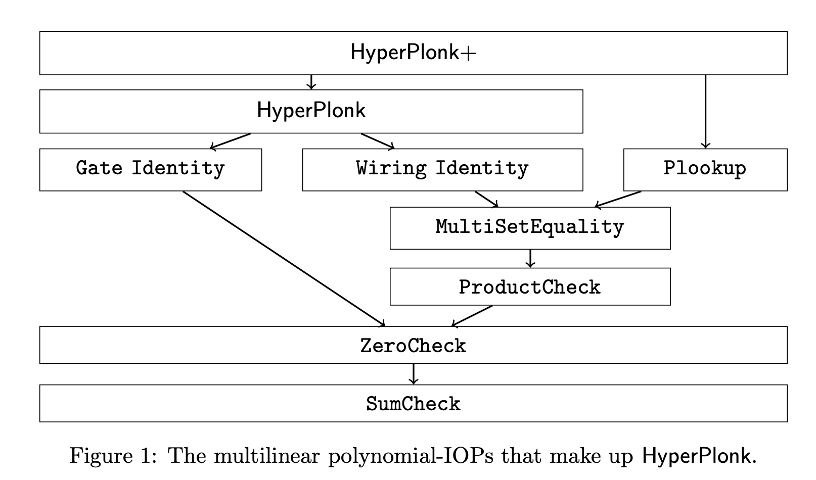
Let $\mathcal C[G]: \mathbb F^{n + m} \rightarrow \mathbb F$ be a circuit with a length-$n$ public input $x \in \mathbb F^n$ and $s$ gates, where each gate can be an addition, multiplication, or a custom gate $G: \mathbb F^2 \rightarrow \mathbb F$. The arithmetization of Plonk converts a circuit into a sequence of $n + s + 1$ triples, i.e., a matrix $\tilde{M} \in \mathbb F^{(n + s + 1) \times 3}$, which represents the execution trace of the circuit. After the commitment to the matrix $\tilde{M}$, the Plonk prover needs to convince the verifier that the committed $\tilde{M}$ satisfies the gate and wiring identities. Hyperplonk follows the paradigm of Plonk, replacing the FFTs in the ZeroCheck part with SumCheck, as shown in Figure 1:

The Computing Components

The current implementation of Hyperplonk is based on Arkworks, which is written in Rust. The following figure illustrates the dependency of components in the Hyperplonk system, where the blocks in gray were implemented in the Hyperplonk paper:

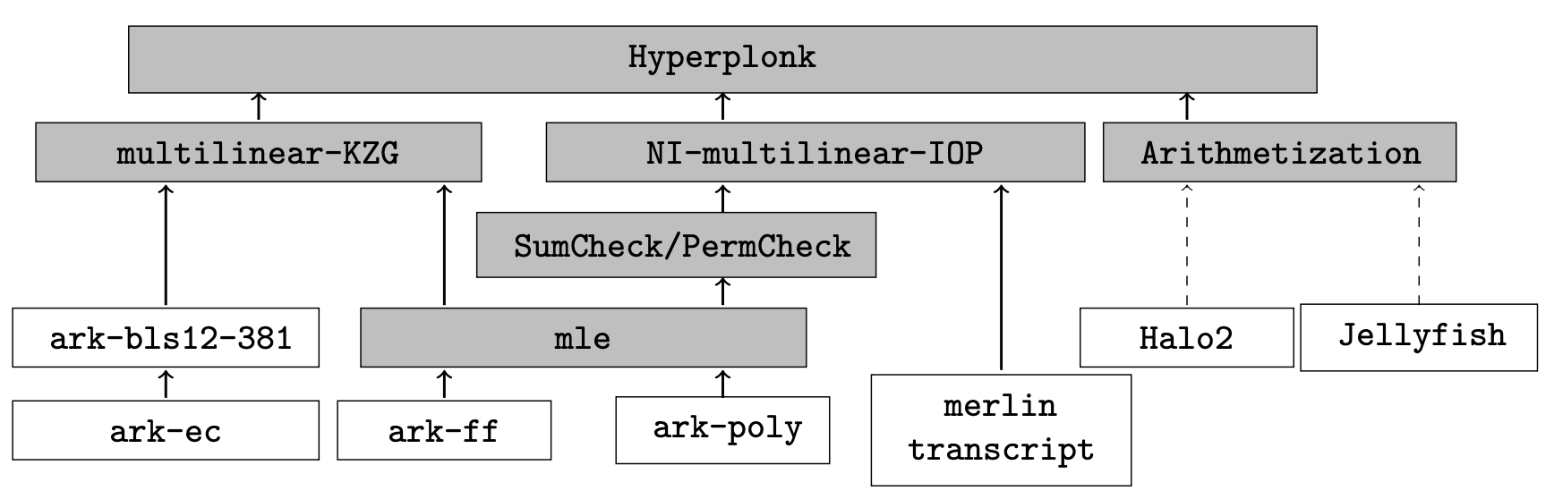
Based on the benchmark of the code for $2^{18}$ constraints (Section 6.2 of Hyperplonk, there are three major computing components:

• Multi-scalar multiplication (MSM): This component is used in the multilinear-KZG commitment and takes about 43.6% of the whole computation.
• Multilinear extension (MLE): This component is used in evaluating multi-linear polynomials in the batching process and takes about 28.5% of the whole computation.
• Sumcheck: This component is used in the multilinear-IOP part to ensure the computation trace is valid and takes about 27.9% of the whole computation.

In the following sections, we will delve into the details of these three components to analyze their hardware-friendliness.

MSM

The MSM component is usually the most time-consuming part in elliptic curve-based SNARKs. Its goal is to compute $Q = \sum_{i = 1}^n x_i G_i$, where $n$ is the size of the MSM, $x_i$ is a 256-bit scalar, and $G_i$ is a point on the curve. The $k_i P_i$ represents the point scalar multiplication (PMULT) of $k_i$ and $P_i$. The Pippenger algorithm is widely used to calculate the MSM problem, which uses some basic arithmetic operations such as point addition (PADD) and point doubling (PDBL). Due to the inherent parallelism of MSM, it is quite friendly to GPU and hardware acceleration. The main difficulty lies in designing a highly efficient modular multiplication component, which is used throughout the proof generation process.

Our FPGA-MSM design is a fully pipelined architecture, which means that in every cycle, the processing element is able to finish a point addition operation. The performance of a fully pipelined architecture is usually bounded by the bandwidth of PCIe. There are three modules in the architecture: the EC point adder, the MSM accumulate table, and the ALU input queue, as shown below:

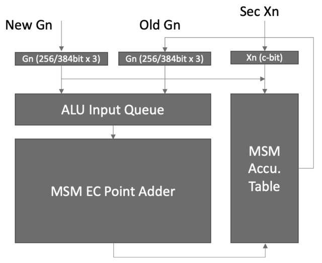
The input to the MSM component consists of the projective coordinates of a point (the length of which depends on the specific curve being used) and a $c$-bit slice of the scalar. The sectional scalar $x_n$ is first checked against the accumulate table to see if it contains the corresponding $G_n$. If it does, then $G_n$ is read out and referred to as the old $G_n$. The new $G_n$ and the old $G_n$ are then sent to the MSM EC point adder to compute their addition, with the result being stored in the accumulation table.

The EC point adder has a very deep pipeline in the circuit, and a related tricky problem is handling read-access to the same table entry before the prior result is written back. A naive approach will introduce stalls and result in suboptimal performance. To address this issue, we implemented dynamic reorder logic using the associative law of point-addition to guarantee that all read-after-write dependencies are correctly handled.

We announced our initial result for the MSM based on a single Xilinx VU13P at the Berkeley ZKP workshop, and now are working on optimizing this part, as well as a highly customized FPGA server. We will announce the performance of MSM on this server soon.

MLE

The task of MLE is to compute the evaluation result for a multilinear polynomial modulo a prime number. The MLE task is parameterized by two things: the number of variables $v$ and the prime number $p$. The input to MLE consists of a sequence of coefficients $\vec{a} = (a_0, a_1,...a_{2^v - 1})$ and a sequence of values $\vec{x} = (x_0, x_1,...x_{v - 1})$, where each number is 256 bits long. The MLE computes the following polynomial:

$f(\vec{a}, \vec{x}) = \sum_{\vec{w} \in \{0, 1\}^v} a_{w_{v - 1},..., w_{0}} \times \prod_{i = 1}^v (x_i w_i + (1 - x_i)(1 - w_i)) \bmod p,$

where $a_{w_{v - 1},..., w_{0}}$ denotes $a_{\sum_{i = 0}^{v - 1} 2^i \cdot w_i}$. For instance, let $v = 2$, the polynomial to be computed is

$f(\vec{a}, \vec{x}) = a_0 \cdot (1 - x_0)(1 - x_1) + a_1 \cdot x_0(1 - x_1) + a_2 \cdot (1 - x_0)x_1 + a_3 \cdot x_0x_1 \cdot.$

If we compute the polynomial directly, we need to deal with $2^v$ terms, each containing a coefficient and $v$ variables, which results in approximately $2^v \cdot v$ multiplications. However, upon closer inspection, we realize that we can merge terms to reduce the number of required multiplications. We can then divide the computation into $v$ layers of multiplication and $v$ layers of addition, which are interleaved. This allows us to reduce the number of needed multiplications to $2^v + 2^{v - 1} + \cdots + 2 = 2 \times (2^v - 1)$, as shown in the following figure:

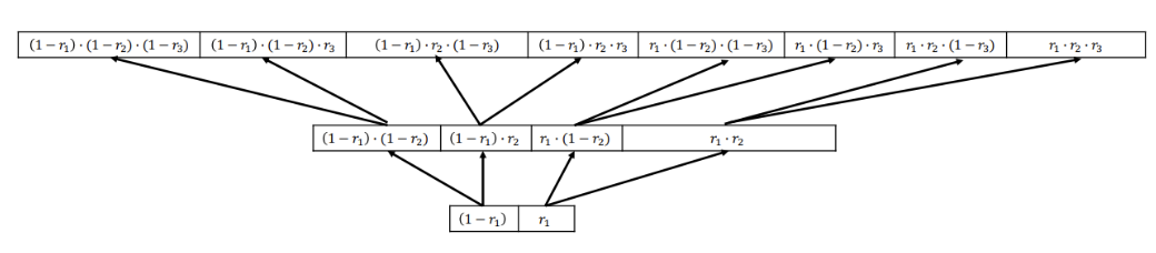
This is a rough outline of how we can use a CPU to compute this polynomial, with each thread computing a single MLE. One disadvantage of this design is the large amount of memory required to store intermediate values. If we try to use this design in hardware acceleration, we will face two problems:

• The on-chip SRAM is not large enough to store intermediate values, so we need to read and write from memory during the computation.
• If we increase parallelism, we may not have enough hardware resources to support so many MLEs.

Our improved design builds on the layered CPU implementation. We noticed that subsequent layers do not need to wait for previous layers to finish; instead, all layers can work simultaneously, connected by queues. The basic module computes $(1 - x_k)a_{left} + x_k a_{right}$, using the merged form as shown in the following diagram:

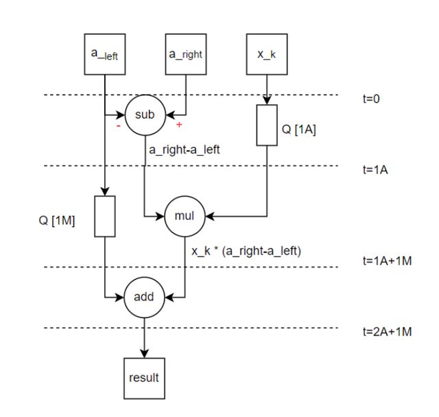
In our initial MLE design, the coefficient vector $(a_0, a_1, \ldots)$ is read in a stream and placed in queue $Q_1$. The $Q_1$ is connected to a basic module that takes two coefficients $(a_{left}, a_{right})$ from $Q_1$ and computes $(1 - x_0)a_{left} + x_0 a_{right}$. The result is placed in queue $Q_2$. Similarly, the $Q_2$ is connected to another basic module that performs the same computation. The result of this module is placed in queue $Q_3$. This process is repeated multiple times until the $v$-th queue. The $v$-th queue $Q_v$ is connected to a basic module that computes and outputs the final result.

Our final design is based on this initial concept, but with several improvements such as multiplexing instead of duplicating the above components. We have expanded it into a fully-pipelined architecture that can handle a 256-bit input at every cycle, similar to our MSM module design. The MLE enjoys hardware-friendness as the MSM module, but the performance is also limited by the bandwidth of the PCIe.

Sumcheck

Essentially, the sumcheck protocol between the prover and verifier is round-dependent, meaning the information exchanged in the current round depends on that of previous rounds. The sumcheck protocol can be made non-interactive using the Fiat-Shamir heuristic, which involves using a hash function to compute the challenge based on the transcript. Omer Shlomovits wrote an excellent post discussing the hardware friendliness of the sumcheck module. We agree with the arguments presented in that post. Given the serial nature of the sumcheck protocol and the hardware-resistant nature of hash functions, it seems difficult to design a hardware acceleration solution that offers significant advantages over CPU/GPU approaches, but we still got inspired by Justin Thaler's tweet about some hardware optimizations for sumcheck.

One potential improvement is to reduce the number of required sumchecks in Hyperplonk. In particular, the paper already mentioned (also in Benedikt Bünz's tweet), that the number of sumchecks can be reduced by batching MLEs. Using this technique, the number of sumchecks is always 2, no matter how complex the custom gate is. Thus the number of sumchecks is much smaller than the number of MLEs.

Conclusions

Compared to the FFT-based SNARK system, the Hyperplonk proof system as it currently stands does not offer significant hardware friendliness. Based on our discussion, the sumcheck module is more hardware unfriendly than the MSM and MLE modules. Novel techniques, either algorithmic or hardware-based, are needed to improve the performance of sumcheck on hardware.

As Omer Shlomovits also mentioned in his post, an alternative approach is to have the hardware-mindset in the design of SNARKs. We tend to agree with this point, not because we are a hardware company, but due to the performance demands of the community. For instance, the hardware-friendness of Hyperplonk can be improved using batching. However, is there a more hardware-friendly variant of Hyperplonk? Stay tuned – we may have a solution!